Understanding the ECO Framework

The Encode-Cluster-Optimize (ECO) framework is the foundation of PyAGC. This tutorial explains how PyAGC’s modular design implements this framework.

The Three Pillars

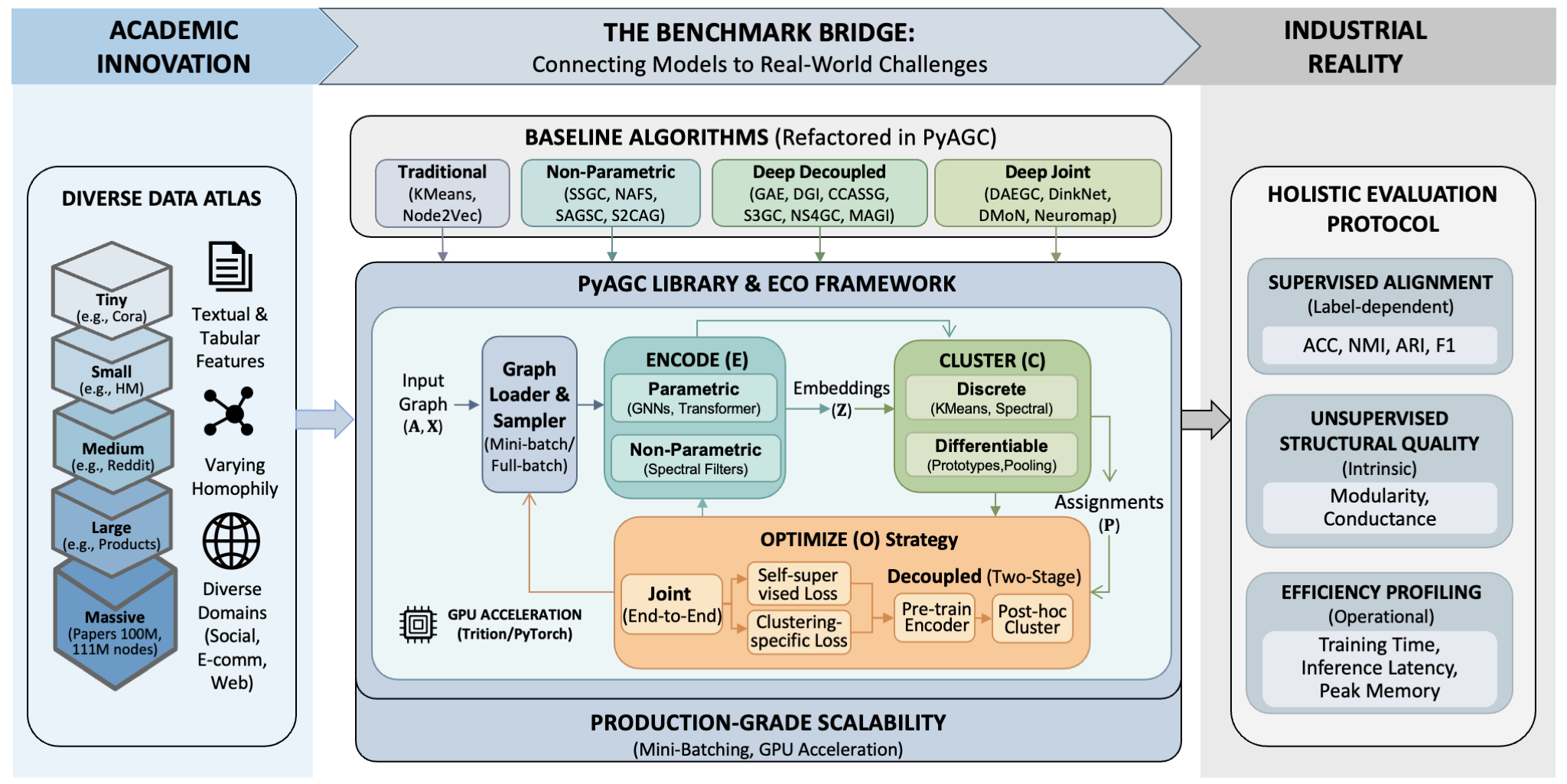
1. Encoder: Learns node representations

2. Cluster Head: Projects embeddings to cluster assignments

3. Optimization Strategy: Defines the training objective and coordination

Encoder Module

The encoder transforms raw graph data into latent representations:

\[\mathbf{Z} = \mathcal{E}(\mathbf{A}, \mathbf{X}; \Theta_{\mathcal{E}})\]

Parametric Encoders

Use learnable graph neural networks:

from pyagc.encoders import create_tuned_gnn
from pyagc.data import get_dataset
from torch_geometric.data import Data

# Load dataset
x, edge_index, y = get_dataset('Cora', root='./data')
data = Data(x=x, edge_index=edge_index)

# Create GCN encoder
gcn_encoder = create_tuned_gnn(
    gnn_type='gcn',
    in_channels=data.num_features,
    hidden_channels=256,
    num_layers=2,
    out_channels=128,
    dropout=0.5,
    norm='batch'
)

# Create GAT encoder with attention
gat_encoder = create_tuned_gnn(
    gnn_type='gat',
    in_channels=data.num_features,
    hidden_channels=256,
    num_layers=2,
    out_channels=128,
    heads=8,
    concat=False,
    dropout=0.6
)

# Forward pass
z = gcn_encoder(data.x, data.edge_index)  # [num_nodes, 128]

Non-Parametric Encoders

Use fixed graph filtering operations without learnable parameters:

from pyagc.models import SSGC
import torch

# Simple Spectral Graph Convolution
# No learnable parameters - purely based on graph structure
model = SSGC(
    alpha=0.05,      # Teleport probability
    K=2,             # Number of propagation steps
    cached=True,     # Cache propagation matrix
    add_self_loops=True
)

# Computes: Z = (I - alpha·D^{-1/2}AD^{-1/2})^K X
# This is a smoothed version of node features
z = model.embed(data.x, data.edge_index)

Cluster Head Module

The cluster head maps embeddings to cluster assignments:

\[\mathbf{P} = \mathcal{C}(\mathbf{Z}; \Theta_{\mathcal{C}})\]

Differentiable Cluster Heads

Allow end-to-end gradient-based training:

from pyagc.clusters import DECClusterHead, DMoNClusterHead

# Get embeddings (assuming z is already computed)
num_nodes, embedding_dim = z.shape
num_clusters = 7

# 1. DEC-style prototype clustering
# Uses Student's t-distribution to compute soft assignments
dec_head = DECClusterHead(
    n_clusters=num_clusters,
    n_features=embedding_dim,
    alpha=1.0  # Degrees of freedom
)

# Initialize cluster centers (e.g., from KMeans)
from pyagc.clusters import TorchKMeans
kmeans = TorchKMeans(n_clusters=num_clusters)
kmeans.fit(z)
dec_head.reset_cluster_centers(kmeans.cluster_centers_)

# Forward: compute clustering loss
loss = dec_head(z)  # KL divergence loss

# Get cluster assignments
clusters = dec_head.cluster(z, soft=False)  # Hard assignments
probs = dec_head.cluster(z, soft=True)      # Soft assignments

# 2. DMoN-style differentiable pooling
# Uses modularity maximization
dmon_head = DMoNClusterHead(
    n_clusters=num_clusters,
    n_features=embedding_dim
)

# Forward: compute modularity and collapse losses
modularity_loss, collapse_loss = dmon_head(z, data.edge_index)
total_loss = modularity_loss + collapse_loss

# Get cluster assignments
clusters = dmon_head.cluster(z, soft=False)

Discrete Cluster Heads

Apply post-hoc clustering algorithms (non-differentiable):

from pyagc.clusters import KMeansClusterHead, TorchKMeans

# 1. Using KMeansClusterHead wrapper
kmeans_head = KMeansClusterHead(
    n_clusters=7,
    backend='torch',  # 'torch' or 'sklearn'
    n_init=10,
    max_iter=300,
    random_state=42
)

# Fit and predict in one step
clusters = kmeans_head.fit_predict(z)

# Or use separately
kmeans_head.fit(z)
clusters = kmeans_head.predict(z)
centers = kmeans_head.cluster_centers_

# 2. Using TorchKMeans directly (GPU-accelerated)
kmeans = TorchKMeans(
    n_clusters=7,
    max_iter=300,
    tol=1e-4,
    random_state=42
)

kmeans.fit(z)
clusters = kmeans.labels_            # [num_nodes]
centers = kmeans.cluster_centers_    # [num_clusters, embedding_dim]
inertia = kmeans.inertia_            # Sum of squared distances

Optimization Strategy

The optimization strategy defines how encoder and cluster head interact during training.

Decoupled Training (Two-Stage)

Pre-train encoder with self-supervised objectives, then apply discrete clustering:

from pyagc.models import NS4GC
from pyagc.data import get_dataset
from pyagc.encoders import create_tuned_gnn
from pyagc.transforms import GSSLTransform
from torch_geometric.data import Data
import torch

# Load data
x, edge_index, y = get_dataset('Cora', root='./data')
data = Data(x=x, edge_index=edge_index)

# Create encoder
encoder = create_tuned_gnn(
    gnn_type='gcn',
    in_channels=data.num_features,
    hidden_channels=64,
    num_layers=2,
    norm='batch'
)

# Create data augmentation
transform1 = GSSLTransform(p_feat_mask=0.2, p_edge_drop=0.3)
transform2 = GSSLTransform(p_feat_mask=0.2, p_edge_drop=0.3)

# Create NS4GC model
model = NS4GC(
    encoder=encoder,
    transform1=transform1,
    transform2=transform2,
    lam=1.0,      # Weight for neighbor loss
    gam=1.0       # Weight for sparsity loss
).to('cuda')

# Stage 1: Pre-train encoder with contrastive learning
# Objective: L_rep = L_ali + λ·L_nei + γ·L_spa
optimizer = torch.optim.Adam(model.parameters(), lr=0.001, weight_decay=0.0)

for epoch in range(200):
    loss = model.train_full(data, optimizer, epoch, verbose=True)

# Stage 2: Generate embeddings and apply KMeans
model.eval()
with torch.no_grad():
    z = model.infer_full(data)  # [num_nodes, hidden_channels]

# Clustering is completely decoupled from encoder training
from pyagc.clusters import KMeansClusterHead
kmeans = KMeansClusterHead(n_clusters=7)
clusters = kmeans.fit_predict(z)

The two stages optimize separate objectives:

\[\text{Stage 1: } \min_{\Theta_{\mathcal{E}}} \mathcal{L}_{\text{rep}}(\mathbf{Z}) = \mathcal{L}_{\text{ali}} + \lambda \mathcal{L}_{\text{nei}} + \gamma \mathcal{L}_{\text{spa}}\]

\[\text{Stage 2: } \min_{\Theta_{\mathcal{C}}} \sum_{i} \|\mathbf{z}_i - \boldsymbol{\mu}_{c_i}\|^2\]

Joint Training (End-to-End)

Train encoder and cluster head together with a combined objective:

from pyagc.models import DAEGC
from pyagc.encoders import create_tuned_gnn
from pyagc.data import get_dataset
from torch_geometric.data import Data
import torch

# Load data
x, edge_index, y = get_dataset('Cora', root='./data')
data = Data(x=x, edge_index=edge_index).to('cuda')

# Get number of clusters
num_clusters = int(y[~torch.isnan(y)].max().item()) + 1

# Create encoder
encoder = create_tuned_gnn(
    gnn_type='gat',
    in_channels=data.num_features,
    hidden_channels=256,
    num_layers=2,
    heads=8,
)

# Create DAEGC model
# Combines GAE reconstruction + DEC clustering
model = DAEGC(
    encoder=encoder,
    n_clusters=num_clusters,
    hidden_channels=256,
    gamma=10.0,           # Weight for clustering loss
    update_interval=5     # Update target distribution every N epochs
).to('cuda')

# Stage 1: Pre-train autoencoder
# Objective: L_pretrain = ||A - decoder(encoder(X, A))||^2
print("Stage 1: Pre-training autoencoder...")
optimizer_pretrain = torch.optim.Adam(
    model.parameters(),
    lr=0.001,
    weight_decay=5e-4
)

for epoch in range(1, 201):
    # Pretrain with reconstruction loss only
    loss = model.train_full(
        data,
        optimizer_pretrain,
        epoch,
        verbose=(epoch % 10 == 0),
        pretrain=True  # Only use reconstruction loss
    )

    if epoch % 50 == 0:
        print(f'Pretrain Epoch {epoch:03d}, Loss: {loss:.4f}')

# Stage 2: Initialize cluster centers using K-Means
print("\nStage 2: Initializing cluster centers with K-Means...")
model.eval()
with torch.no_grad():
    # Get pretrained embeddings
    z = model.embed(data.x, data.edge_index)
    # Normalize for better clustering
    z = torch.nn.functional.normalize(z, p=2, dim=1)

# Initialize cluster centers via K-Means
from pyagc.clusters import TorchKMeans
kmeans = TorchKMeans(n_clusters=num_clusters, random_state=42)
kmeans.fit(z)

# Set initialized centers to the DEC cluster head
model.cluster_head.reset_cluster_centers(kmeans.cluster_centers_)
print(f"✓ Cluster centers initialized: {model.cluster_head.cluster_centers.shape}")

# Stage 3: Joint fine-tuning
# Objective: L_total = L_reconstruction + γ·KL(P || Q)
print("\nStage 3: Joint fine-tuning with clustering loss...")
optimizer_finetune = torch.optim.Adam(
    model.parameters(),
    lr=0.0001,
    weight_decay=0.0
)

for epoch in range(1, 201):
    # Joint training with both reconstruction and clustering losses
    loss = model.train_full(
        data,
        optimizer_finetune,
        epoch,
        verbose=(epoch % 10 == 0),
        pretrain=False  # Use both reconstruction + clustering losses
    )

    if epoch % 10 == 0:
        print(f'Finetune Epoch {epoch:03d}, Loss: {loss:.4f}')

# Get final cluster assignments
model.eval()
clusters = model.infer_full(data)  # Hard cluster assignments

The joint loss simultaneously optimizes representation and clustering:

\[\min_{\Theta_{\mathcal{E}}, \Theta_{\mathcal{C}}} \mathcal{L}_{\text{total}} = \underbrace{\|\mathbf{A} - \sigma(\mathbf{Z})\|^2}_{\text{reconstruction}} + \gamma \underbrace{\text{KL}(\mathbf{P} \| \mathbf{Q})}_{\text{clustering}}\]

Composing ECO Components

PyAGC’s modular design enables flexible composition of components.

Example 1: Custom Model with Swappable Encoders

from pyagc.models import ClusteringModel, LossOutput
from pyagc.encoders import create_tuned_gnn
from pyagc.clusters import DECClusterHead

class MyClusteringModel(ClusteringModel):
    """Custom clustering model with flexible encoder."""

    def __init__(self, in_channels, hidden_channels, num_clusters,
                 gnn_type='gcn'):
        super().__init__()

        # Easily swap between different GNN types
        self.encoder = create_tuned_gnn(
            gnn_type=gnn_type,  # Try: 'gcn', 'gat', 'sage', 'gin'
            in_channels=in_channels,
            hidden_channels=hidden_channels,
            num_layers=2,
            out_channels=128
        )

        self.cluster_head = DECClusterHead(
            n_clusters=num_clusters,
            n_features=128
        )

    def forward(self, data):
        z = self.encoder(data.x, data.edge_index)
        return z

    def loss(self, data):
        z = self.forward(data)
        cluster_loss = self.cluster_head(z)
        return LossOutput(total=cluster_loss)

    def predict(self, data):
        z = self.forward(data)
        return self.cluster_head.cluster(z, soft=False)

# Use different encoders with same model structure
model_gcn = MyClusteringModel(1433, 256, 7, gnn_type='gcn')
model_gat = MyClusteringModel(1433, 256, 7, gnn_type='gat')
model_sage = MyClusteringModel(1433, 256, 7, gnn_type='sage')

Example 2: Comparing Different Cluster Heads

from pyagc.clusters import (
    DECClusterHead,
    DMoNClusterHead,
    KMeansClusterHead,
    DinkClusterHead
)

# Shared encoder for fair comparison
encoder = create_tuned_gnn('gcn', data.num_features, 256, 2)

# Get embeddings once
with torch.no_grad():
    z = encoder(data.x, data.edge_index)

# Compare different clustering approaches

# 1. DEC: Prototype-based with Student's t-distribution
dec_head = DECClusterHead(n_clusters=7, n_features=256)
dec_head.reset_cluster_centers()  # Random init or use KMeans
clusters_dec = dec_head.cluster(z, soft=False)

# 2. DMoN: Modularity-aware differentiable pooling
dmon_head = DMoNClusterHead(n_clusters=7, n_features=256)
clusters_dmon = dmon_head.cluster(z, soft=False)

# 3. DinkNet: Dilation and shrink regularization
dink_head = DinkClusterHead(n_clusters=7, n_features=256)
clusters_dink = dink_head.cluster(z, soft=False)

# 4. KMeans: Classic centroid-based
kmeans_head = KMeansClusterHead(n_clusters=7)
clusters_kmeans = kmeans_head.fit_predict(z)

# Evaluate all methods
from pyagc.metrics import label_metrics
for name, clusters in [
    ('DEC', clusters_dec),
    ('DMoN', clusters_dmon),
    ('DinkNet', clusters_dink),
    ('KMeans', clusters_kmeans)
]:
    results = label_metrics(y, clusters, metrics=['NMI', 'ARI', 'ACC'])
    print(f"{name:8s} - NMI: {results['NMI']:.4f}, "
          f"ARI: {results['ARI']:.4f}, ACC: {results['ACC']:.4f}")

Example 3: Custom Multi-Objective Optimization

from pyagc.models import TrainableModel, LossOutput
from pyagc.encoders import create_tuned_gnn
from pyagc.clusters import DECClusterHead
import torch
import torch.nn.functional as F

class MultiObjectiveModel(TrainableModel):
    """Custom model with multiple loss components."""

    def __init__(self, in_channels, hidden_channels, num_clusters):
        super().__init__()

        self.encoder = create_tuned_gnn(
            gnn_type='gcn',
            in_channels=in_channels,
            hidden_channels=hidden_channels,
            num_layers=2,
            out_channels=128
        )

        self.cluster_head = DECClusterHead(
            n_clusters=num_clusters,
            n_features=128,
            alpha=1.0
        )

        # Decoder for reconstruction
        self.decoder = torch.nn.Linear(128, in_channels)

    def forward(self, data):
        z = self.encoder(data.x, data.edge_index)
        return z

    def loss(self, data):
        z = self.forward(data)

        # 1. Clustering loss (KL divergence)
        loss_cluster = self.cluster_head(z, update_target=True)

        # 2. Reconstruction loss
        x_recon = self.decoder(z)
        loss_recon = F.mse_loss(x_recon, data.x)

        # 3. Contrastive loss (InfoNCE-style)
        # Normalize embeddings
        z_norm = F.normalize(z, p=2, dim=1)
        # Compute similarity matrix
        sim_matrix = torch.matmul(z_norm, z_norm.t()) / 0.5
        # Create positive pairs from neighbors
        adj = torch.sparse_coo_tensor(
            data.edge_index,
            torch.ones(data.edge_index.shape[1], device=z.device),
            (data.num_nodes, data.num_nodes)
        ).to_dense()
        # Positive pairs: neighbors in graph
        pos_mask = adj > 0
        # Negative pairs: non-neighbors
        neg_mask = ~pos_mask
        neg_mask.fill_diagonal_(False)

        # Compute contrastive loss
        pos_sim = sim_matrix[pos_mask].mean() if pos_mask.sum() > 0 else 0
        neg_sim = torch.logsumexp(sim_matrix[neg_mask], dim=0).mean()
        loss_contrast = -pos_sim + neg_sim

        # 4. Regularization: encourage balanced clusters
        q = self.cluster_head.cluster(z, soft=True)
        cluster_sizes = q.sum(dim=0)
        target_size = q.shape[0] / q.shape[1]
        loss_balance = F.mse_loss(cluster_sizes,
                                 torch.full_like(cluster_sizes, target_size))

        # Combined loss with weights
        total_loss = (loss_cluster +
                     0.1 * loss_recon +
                     0.05 * loss_contrast +
                     0.01 * loss_balance)

        return LossOutput(
            total=total_loss,
            loss_cluster=loss_cluster,
            loss_recon=loss_recon,
            loss_contrast=loss_contrast,
            loss_balance=loss_balance
        )

    def predict(self, data):
        z = self.forward(data)
        return self.cluster_head.cluster(z, soft=False)

# Train the model
model = MultiObjectiveModel(
    in_channels=data.num_features,
    hidden_channels=256,
    num_clusters=7
).to('cuda')

optimizer = torch.optim.Adam(model.parameters(), lr=0.001)

for epoch in range(200):
    loss_output = model.train_full(data, optimizer, epoch)

    if epoch % 10 == 0:
        print(f'Epoch {epoch:03d}:')
        print(f'  Total: {loss_output.total:.4f}')
        print(f'  Cluster: {loss_output.loss_cluster:.4f}')
        print(f'  Recon: {loss_output.loss_recon:.4f}')
        print(f'  Contrast: {loss_output.loss_contrast:.4f}')
        print(f'  Balance: {loss_output.loss_balance:.4f}')

Example 4: Mini-Batch Training for Large Graphs

from torch_geometric.loader import NeighborLoader

# For large graphs, use mini-batch training
train_loader = NeighborLoader(
    data,
    num_neighbors=[15, 10],  # 2-layer sampling
    batch_size=1024,
    shuffle=True,
    num_workers=4
)

# Create model
model = NS4GC(
    encoder=encoder,
    transform1=transform1,
    transform2=transform2
).to('cuda')

optimizer = torch.optim.Adam(model.parameters(), lr=0.001)

# Train with mini-batches
for epoch in range(200):
    avg_loss = model.train_batch(train_loader, optimizer, epoch)

    if epoch % 10 == 0:
        print(f'Epoch {epoch:03d}, Loss: {avg_loss:.4f}')

# Inference can still use full-batch or mini-batch
inference_loader = NeighborLoader(
    data,
    num_neighbors=[-1],  # Sample all neighbors
    batch_size=2048,
    shuffle=False
)

z = model.infer_batch(inference_loader)

ECO Taxonomy of Methods

PyAGC organizes 20+ state-of-the-art algorithms into the ECO framework:

Method	Encoder	Cluster Head	Optimization	Key Innovation
KMeans	None	Discrete	N/A	Attribute-only baseline
Node2Vec	Non-param	Discrete	Decoupled	Structure-only baseline
SSGC	Non-param	Discrete	Decoupled	Markov diffusion-based spectral filtering
NAFS	Non-param	Discrete	Decoupled	Adaptive filter selection with ensemble
SAGSC	Non-param	Discrete	Decoupled	Graph regularized subspace clustering
S2CAG	Non-param	Discrete	Decoupled	Conductance minimization for subspace clustering
MS2CAG	Non-param	Discrete	Decoupled	Modularity maximization for subspace clustering
GAE/VGAE	Parametric	Discrete	Decoupled	Graph autoencoder with optional variational
ARGA/ARGVA	Parametric	Discrete	Decoupled	Adversarially regularized GAE/VGAE
DGI	Parametric	Discrete	Decoupled	Mutual information maximization
CCASSG	Parametric	Discrete	Decoupled	Canonical correlation for redundancy reduction
GBT	Parametric	Discrete	Decoupled	Barlow Twins for redundancy reduction
S3GC	Parametric	Discrete	Decoupled	Scalable contrastive learning
NS4GC	Parametric	Discrete	Decoupled	Node similarity preserving contrastive
MAGI	Parametric	Discrete	Decoupled	Modularity-aware contrastive clustering
DAEGC	Parametric	Differentiable	Joint	GAT + DEC clustering
DinkNet	Parametric	Differentiable	Joint	Dilation and shrink regularization
MinCut	Parametric	Differentiable	Joint	Spectral cut minimization
DMoN	Parametric	Differentiable	Joint	Modularity maximization
Neuromap	Parametric	Differentiable	Joint	Neural map equation
GCSBM	Parametric	Differentiable	Joint	Stochastic block model

Conclusion

The ECO framework provides a unified lens for understanding and implementing attributed graph clustering methods. By decomposing algorithms into Encoder, Cluster Head, and Optimization Strategy components, PyAGC enables:

• ✅ Modularity: Swap components without rewriting code

• ✅ Extensibility: Easy to add new encoders, cluster heads, or optimization strategies

• ✅ Reproducibility: Standardized evaluation protocols and benchmarking

• ✅ Scalability: Support for graphs from thousands to billions of nodes

• ✅ Flexibility: From research prototyping to production deployment

Start experimenting with the ECO framework today and build state-of-the-art graph clustering solutions!

Next Steps

• Create a custom cluster head for novel objectives

• Scale to massive graphs with mini-batch training